Introduction to Knowledge Distillation

Knowledge Distillation (KD) is a model compression technique, popularized by Hinton et al. in their 2015 paper “Distilling the Knowledge in a Neural Network”. The core idea is to transfer (or “distill”) the knowledge from a large, complex model (the “teacher”) to a smaller, simpler model (the “student”), enabling efficient deployment without significant loss in performance.

Today we will discuss the background and motivation of KD, and followed by the methodology, and finally we will dive deep into the terminology “temperature” specifically —- We know that “distiallation” should be done under high temperature, then what does “temperature” represents and how to pick the most appropriate temperature?

1. Introduction

Why We Need Large Models?

We can view underfitting and overfitting through the relative relationship between model size and training data size. AI scientists are likely familiar with this, but for beginners, here is a vivid analogy that my colleague once shared (and it left a deep impression on me):

A model is like a container, and the knowledge contained in the training data is like water poured into it. When the amount of knowledge (water) exceeds what the model can represent (the container’s volume), adding more data does not improve performance (extra water cannot fit into the container). This corresponds to underfitting, as the model’s representational capacity is limited. Conversely, when the model size exceeds the representational needs of the available knowledge (a container larger than the water it holds), the result is overfitting. The model’s variance increases (imagine shaking a half-full container—the water sloshes around unstably).

We need large models because We have so much knowledge to learn! But as models get larger and more powerful, it also brings practical costs (latency, memory, energy).

Why We Need Model Compression?

Although in general we do not deliberately distinguish between models used in training and those used in deployment, there actually exists a certain inconsistency between the two:

During training, we rely on complex models and significant computational resources in order to extract information from very large and highly redundant datasets. The models that achieve the best performance are often very large, sometimes even ensembles of multiple models. However, such large models are inconvenient for deployment in production services, mainly due to the following bottlenecks:

• Slow inference speed
• High resource requirements (memory, GPU memory, etc.)
• Strict constraints on latency and computational resources at deployment time

Because of this, model compression (reducing the number of model parameters while preserving performance) has become an important problem. Knowledge Distillation is one such model compression method.

The Actual Relationship Between Model Size and Capacity

The container-and-water analogy above is classic and fitting, but it can also lead to a misunderstanding:
People might intuitively think that to preserve a similar amount of knowledge, one must also preserve a model of a similar scale. In other words, the number of parameters in a model essentially determines how much “knowledge” from the data it can capture.

This way of thinking is mostly correct, but there are some important caveats:

1. The relationship between a model size and the amount of “knowledge” it can capture is not a stable linear one (curve ① in the figure below). Instead, it more closely follows a growth curve with diminishing marginal returns (curves ② and ③).
2. Even with the same architecture and the same number of parameters, trained on the same dataset, the amount of knowledge a model can capture is not necessarily identical. Another crucial factor is the training method. With appropriate training, a model with relatively fewer parameters can still capture more knowledge (as shown by the comparison between curves ③ and ②).

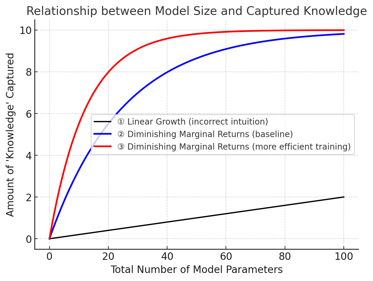
Figure 1: The relationship between model size and knowledge capacity: as model size increases, the amount of knowledge it can capture grows, but with diminishing returns.

2. Theoretical Basis of Knowledge Distillation

The Framework: Teacher-Student

Knowledge Distillation adopts a Teacher–Student framework, where the Teacher acts as the producer of knowledge, and the Student acts as the receiver of knowledge. The distillation process consists of two stages:

1. Training the Teacher Model (Net-T):

   • The Teacher is a relatively complex model, possibly even an ensemble of multiple separately trained models.
   • There are no restrictions on its architecture, parameter count, or whether it is an ensemble.
   • The only requirement is that for an input (X), it outputs (Y), where (Y) is mapped through a softmax layer to produce probabilities for each class.

2. Training the Student Model (Net-S):

   • The Student is a single model with fewer parameters and a simpler structure.
   • For the same input (X), it also outputs (Y), which after softmax corresponds to class probabilities.

In this paper, the problem is restricted to classification tasks, or other problems that are essentially classification in nature (e.g. generation task). These problems all share a common feature: the model ends with a softmax layer, whose output corresponds to the probability of each class.

Why Knowledge Distillation?

If we return to the most fundamental theory of machine learning, we are reminded of a core point (often overlooked once we dive deeper into technical details):

The ultimate purpose of machine learning is to train a model with strong generalization ability for a given problem.

• Strong generalization ability means that the model can reliably capture the relationship between inputs and outputs across all data for the problem — whether it is training data, test data, or unseen data that belongs to the same distribution.

In practice, however, we cannot possibly collect all data for a problem. New data is always being generated. As a result, our training objective shifts: instead of modeling the complete input–output relationship, we settle for approximating it using the training dataset, which is merely a sample of the true data distribution.
Therefore, the optimal solution learned on the training set will almost inevitably deviate from the true global optimum (ignoring model capacity considerations here).

In the case of Knowledge Distillation, since we already have a Teacher model (Net-T) with strong generalization ability, we can leverage it to train the Student (Net-S). This allows the Student to directly learn the Teacher’s generalization capability.

A simple and effective way to transfer this generalization ability is to use the probabilities output by the Teacher’s softmax layer as soft targets for the Student.

Comparison between KD Training and Traditional Training

• Traditional training (hard targets):
  Maximize the likelihood of the ground truth label.

• Knowledge Distillation training (soft targets):
  Use the class probabilities from a large Teacher model as soft targets.

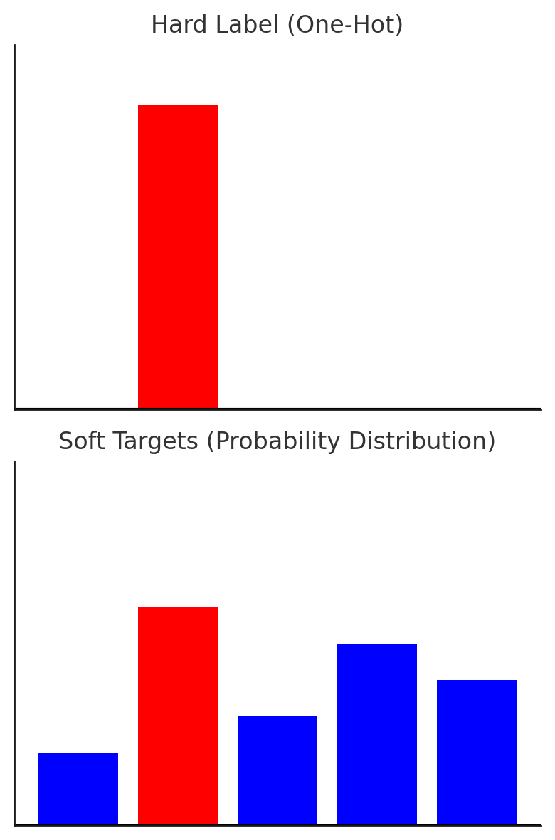
Figure 2: Up - Hard Target; Down - Soft Target

Why is KD Training More Effective?

The output of the softmax layer contains far more information than just the positive (correct) label.

• Even among the negative labels, their probabilities carry meaningful differences — for example, some negative classes may have much higher probabilities than others.
• In contrast, in traditional training with hard targets, all negative labels are treated equally (probability = 0).

In other words, KD training provides richer information per sample to the Student model (Net-S), compared to traditional hard-target training.

An Example: Handwritten digit classification

In the handwritten digit classification task MNIST, the output classes are 10 (digits 0–9).

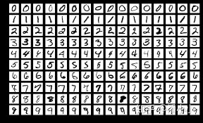
Figure 3: MNIST -- hand-writing digit classification task

Suppose an input digit “2” looks more like a “3”

• In this case, the softmax output might assign a probability of 0.1 to class “3,” while the other negative classes receive very small probabilities.

Now consider another digit “2” that looks more like a “7”

• Here, the softmax output might assign a probability of 0.1 to class “7”

Although both samples have the same hard target (the true label is “2”), their soft targets differ. This shows that soft targets carry more information than hard targets.

Furthermore, when the entropy of the soft target distribution is relatively high, the soft targets contain richer knowledge.

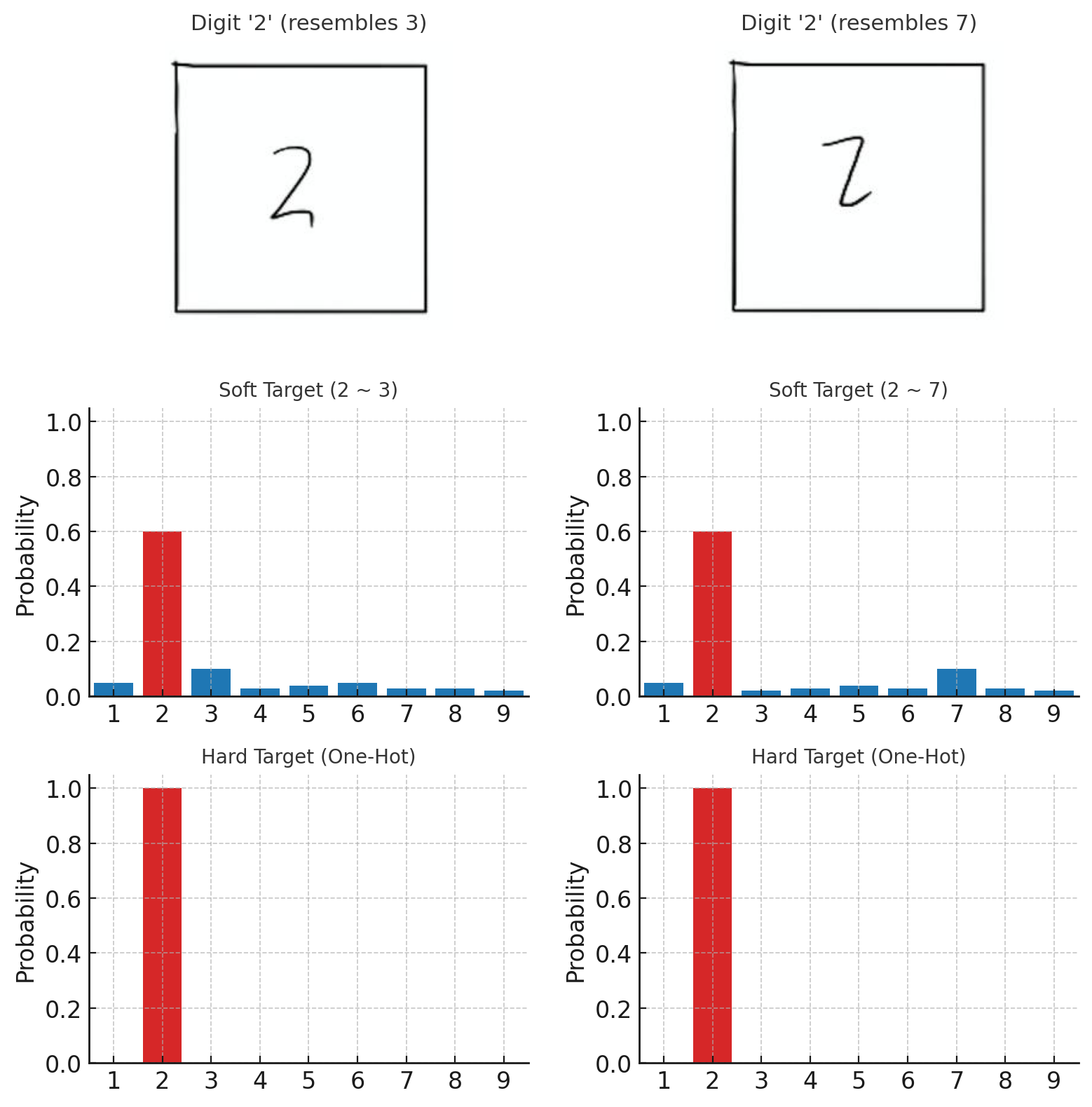
Figure 4: Hard targets of the two '2' are the same while soft targets are different

This explains why a Student model (Net-S) trained through knowledge distillation achieves stronger generalization ability compared to a model trained with the same architecture and training data but only using hard targets.

Introduct of Temperature (T)

Let’s first recall the original softmax function:

$$ q_i=\frac{\exp(z_i)}{\sum_j \exp(z_j)} $$ where $z_i$ is the logit value of class i, and $q_i$ is the probability of class i: $\sum_i q_i = 1$.

If we directly use the softmax outputs as soft targets, there is a problem:
when the softmax distribution is too sharp (low entropy), the probabilities of the negative classes are all near zero and contribute almost nothing to the loss—so little that they can be ignored.
This is where the temperature variable becomes useful.

With temperature T, the softmax becomes:

$$ q^T_i=\frac{\exp(z_i/T)}{\sum_j \exp(z_j/T)} $$

• Here, T is the temperature.
• The original softmax is the special case (T=1).
  As T increases, the output probability distribution becomes smoother (higher entropy). The information carried by negative classes is amplified relatively, causing training to pay more attention to the negatives.

3. Methodology of Knowledge Distillation

General KD Procedure

• Step 1: Train the Teacher model (Net-T).
• Step 2: At a higher temperature T, distill the knowledge from Net-T into the Student model (Net-S). We feed the same transfer set to Net-T and Net-S (we can simply reuse the training set used for Net-T).
• Step 3: After Net-S has finished training, its softmax temperature should be reset to (T = 1) during inference.

Training Net-T is straightforward, so we focus on Step 2: high-temperature distillation.
In this step, the objective for Net-S is a weighted sum of:

• Distillation loss — compares the Student’s outputs to the Teacher’s soft targets (softmax with temperature T), and
• Hard loss — the usual supervised loss against hard targets (ground truth).

Figure 5: Knowledge Distillation Diagram (from https://intellabs.github.io/distiller/knowledge_distillation.html)

Loss Function of Knowledge Distillation

The loss function used in knowledge distillation stage is formally $$ L=\alpha L_{\text{soft}}+\beta L_{\text{hard}} $$

Notation

• $v_i$: logits of Net-T (Teacher)
• $z_i$: logits of Net-S (Student)
• $p_i^{T}$: Teacher’s softmax output at temperature $T$ for class $i$
• $q_i^{T}$: Student’s softmax output at temperature $T$ for class $i$
• $c_i$: ground-truth indicator for class $i$, $c_i \in {0,1}$ (1 = positive class, 0 = otherwise)
• $N$: number of classes

Using Net-T’s high-temperature softmax distribution as the soft target, the cross-entropy between Net-S’s softmax at the temperature T and the soft target is distillation loss: $L_{\text{soft}}$.

$$ L_{\text{soft}} = - \sum_{j=1}^{N} p_j^{T}\log\big(q_j^{T}\big), $$

$\text{where}$

$$ p_i^{T} = \frac{e^{v_i/T}}{\sum_{k=1}^{N} e^{v_k/T}}, \qquad q_i^{T} = \frac{e^{z_i/T}}{\sum_{k=1}^{N} e^{z_k/T}}. $$

The cross-entropy between Net-S’s standard softmax output (i.e., $T=1$) and the ground truth is the second part of the hard loss: $L_{\text{hard}}$.

$$ L_{\text{hard}} = - \sum_{j=1}^{N} c_j \log\big(q_j^{1}\big), \quad\text{where}\quad q_i^{1}=\frac{e^{z_i}}{\sum_{k=1}^{N} e^{z_k}}. $$

Why include $L_{\text{hard}}$?

Net-T is not error-free. Using the ground truth helps prevent the Student from inheriting the Teacher’s occasional mistakes.
Analogy: A teacher is far more knowledgeable than a student, yet can still be wrong at times. If the student also consults the answer key in addition to the teacher’s guidance, they are less likely to be misled by those rare errors.

Why scaling distillation loss by $T^2$?

Quick Answer: In knowledge distillation, the gradient from the distillation loss scales in a magnitude of $1/T^2$ of that from hard loss. That’s why we multiply the distillation loss by $T^2$ to keep gradient magnitudes comparable.

The distillation loss $L_{\text{soft}}$ (cross-entropy with soft targets) is

$$ L_{\text{soft}} = -\sum_i p^T_i \log q^T_i. $$

The hard loss $L_{\text{hard}}$ is

$$ L_{\text{hard}} = - \sum_{j=1}^{N} c_j \log\big(q_j^{1}\big) $$

In back propagation, the chain rule propagates gradients from the loss $L_{\text{soft}}$ and $L_{\text{hard}}$ back through every operation.

$$ \frac{\partial L_{\text{soft}}}{\partial \theta} = \sum_k \big( \sum_i \frac{\partial L_{\text{soft}}}{\partial q_i^T} \cdot \frac{\partial q_i^T}{\partial z_k} \big) \cdot \frac{\partial z_k}{\partial \theta} $$

$$ \frac{\partial L_{\text{hard}}}{\partial \theta} = \sum_k \big( \sum_j \frac{\partial L_{\text{hard}}}{\partial q_j^1} \cdot \frac{\partial q_j^1}{\partial z_k} \big) \cdot \frac{\partial z_k}{\partial \theta} $$

Since the third terms in both gradient formula are identical, so we need to analyze the impact from $L_{\text{soft}}$ and $L_{\text{hard}}$ respectively on each logit $z_k$ (the first two terms)

Using the softmax-with-temperature Jacobian, since $q^T_i=\frac{\exp(z_i/T)}{\sum_j \exp(z_j/T)}$

$$ \frac{\partial L_{\text{soft}}}{\partial q^T_i} = -\frac{1}{T} \cdot \frac{p_i^T}{q_{i}^T} $$

$$ \frac{\partial q^T_i}{\partial z_k} = \frac{1}{T} q^T_i\left(\delta_{ik} - q_{k}^T\right) $$ $$ \frac{\partial L_{\text{hard}}}{\partial q_j^1} = -\frac{c_j}{q_j^1} $$

$$ \frac{\partial q_j^1}{\partial z_k} = q_j^1\big(\delta_{jk} - q_k^1\big) $$

$\delta_{ik}$ is Kronecker delta, defined as:

$$ \delta_{ik} = \begin{cases} 1 & \text{if } i = k \\ 0 & \text{if } i \neq k \end{cases} $$

Now the gradient component of the loss $L$ (a scalar) with respect to the logit of class k $z_k$ is

$$ \frac{\partial L_{\text{soft}}}{\partial z_k} = \sum_i\frac{\partial L_{\text{soft}}}{\partial q^T_i} \frac{\partial q^T_i}{\partial z_k} = -\frac{1}{T} \sum_i p_i^T \left(\delta_{ik} - q_{k}^T\right) = \frac{1}{T}\left(q_k^T - p_k^T\right) $$

$$\frac{\partial L_{\text{hard}}}{\partial z_k} = \sum_j\frac{\partial L_{\text{hard}}}{\partial q^1_j} \frac{\partial q^1_j}{\partial z_k} = - \sum_j c_j \left(\delta_{jk} - q_{k}^1\right) = q_k^1 - c_k$$

First-Order Taylor Expansion of the Probability Gap

Conclusion: The gap $\big(q_k^{T} - p_k^{T}\big)$ itself shrinks as $1/T$ compared to $\big(q_k^{1} - p_k^{1}\big)$.

Let the teacher logits be $v$ and the student logits be $z = v + \Delta z$ with a small difference $\Delta z$.
The softened probabilities at temperature $T$ are

The Problem

We denote $$ p^{(T)} = \text{softmax}\left(\tfrac{v}{T}\right) \qquad q^{(T)} = \text{softmax}\left(\tfrac{z}{T}\right) $$ We want to approximate the gap $q^{(T)} - p^{(T)}$.

Recap:

$$ p_k^{T}=\frac{e^{v_k/T}}{\sum_{i=1}^{N} e^{v_i/T}} = \text{softmax}(v_k/T) \\ q_k^{T}=\frac{e^{z_k/T}}{\sum_{i=1}^{N} e^{z_i/T}} = \text{softmax}(z_k/T) $$

Reformulation

Let

$$ s = \frac{v}{T}, \Delta s = \frac{\Delta z}{T} $$

Then $$ q^{(T)} = \text{softmax}(s + \Delta s), \quad p^{(T)} = \text{softmax}(s) $$

Expand $\text{softmax}(s + \Delta s)$ around $s$:

$$ \text{softmax}(s + \Delta s) \approx \text{softmax}(s) + J(s)\Delta s $$

where $J(s)$ is the Jacobian of softmax at $s$.

Thus,

$$ q^{(T)} - p^{(T)} \approx J\left(\tfrac{v}{T}\right)\frac{\Delta z}{T}. $$

Since $J(\cdot)$ is $O(1)$, the gap scales as

$$ q^{(T)} - p^{(T)} = O\left(\tfrac{1}{T}\right) $$

Combining the two factors

From (1): $$ \frac{\partial L_{\text{soft}}}{\partial z_k} = \frac{1}{T}\left(q_k^T - p_k^T\right) = \frac{1}{T}\cdot O\left(\frac{1}{T}\right) = O\left(\frac{1}{T^2}\right). $$

Therefore, the gradient magnitude from soft targets scales as $1/T^2$.

4. A Special Case: Directly Matching Logits (without softmax)

“Directly matching logits” means we use the inputs to softmax (logits)—not the softmax outputs—as the soft targets, and minimize the squared difference between the Teacher’s and Student’s logits.

Takeaway: Directly matching logits is the $T \to \infty$ special case of high-temperature distillation.

For a single example, the gradient of the distillation loss with respect to the Student logit $z_k$ is

$$ \frac{\partial L_{\text{soft}}}{\partial z_k} = \frac{1}{T}\left(q_k^T - p_k^T\right) = \frac{1}{T}\left(\frac{e^{z_k/T}}{\sum_j e^{z_j/T}}-\frac{e^{v_i/T}}{\sum_j e^{v_j/T}}\right) $$

When $T \to \infty$, use the approximation $e^{x/T} \approx 1 + \frac{x}{T}$. Then

$$ \frac{\partial L_{\text{soft}}}{\partial z_k} \approx \frac{1}{T}\left(\frac{1+ z_k/T}{N + \sum_j z_j/T}-\frac{1+ v_i/T}{N + \sum_j v_j/T}\right). $$

If we further assume the logits are zero-mean per example,

$$ \sum_j z_j = \sum_j v_j = 0, $$

the expression simplifies to

$$ \frac{\partial L_{\text{soft}}}{\partial z_k} \approx \frac{1}{N T^{2}}(z_k - v_k). $$

This is equivalent (up to a constant factor) to minimizing the squared error between logits:

$$ L_{\text{MSE}} = \frac{1}{N}(z_k - v_k)^2 $$

5. Discussion of “Temperature”

Question: We know “distillation” is performed at a high temperature.
What exactly does this “temperature” represent, and how should we tune it?

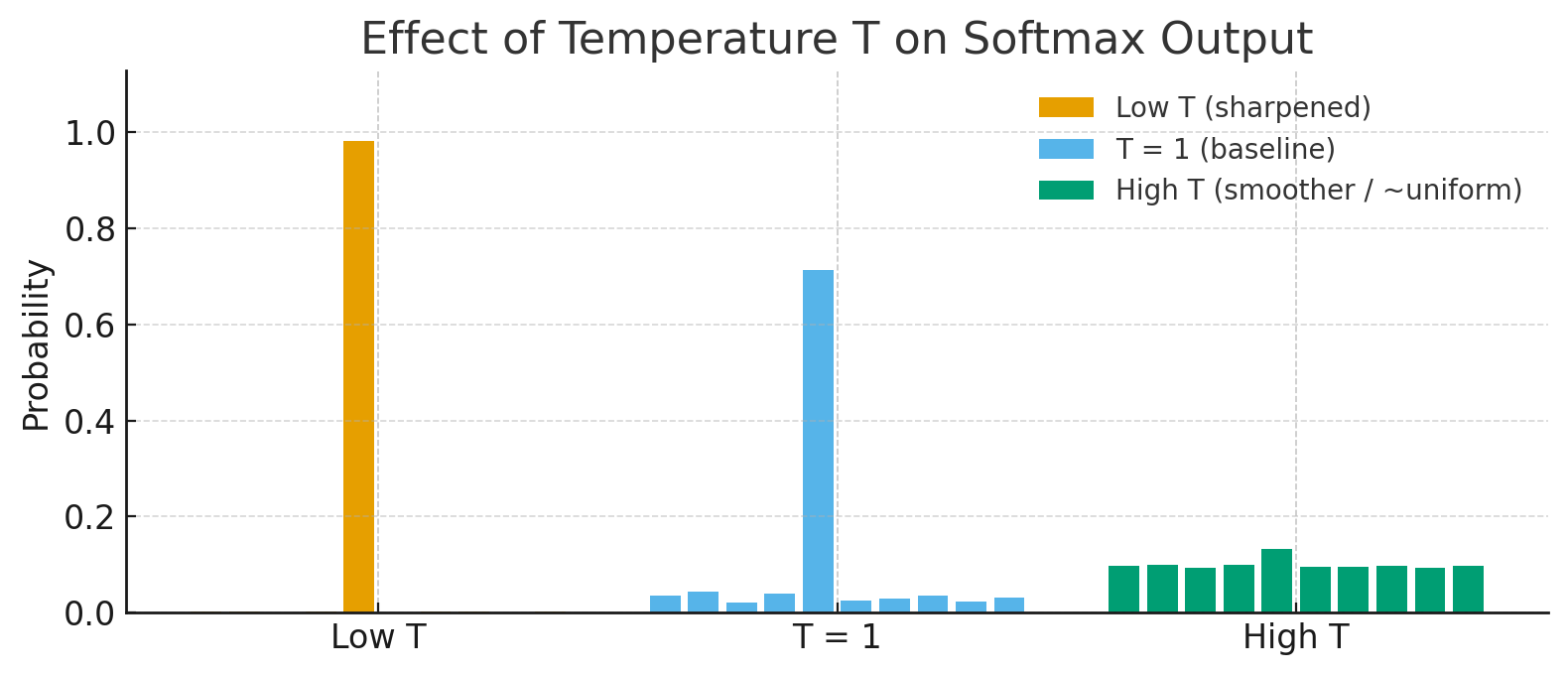
Figure 6: As the temperature T increases, the entropy of the probability distribution increases.

Characteristics of Temperature

Recall softmax with temperature T:

$$ q_i^T = \frac{\exp(z_i/T)}{\sum_j \exp(z_j/T)}. $$

• The standard softmax is the special case (T=1).
  When T<1, the distribution becomes sharper/steeper;
  when T>1, it becomes smoother/flatter.

• As T increases, the probabilities tend toward being more uniform.
  In the extremes:
  (i) $T \to \infty$: softmax approaches a uniform distribution;
  (ii) $T \to 0^+$: softmax approaches an argmax/one-hot distribution.

• Regardless of the value of T, soft targets still tend to underweight the information in very small probabilities $q_i$ (they contribute little signal).

What Does Temperature Represent, and How to Choose It?

• The temperature controls how much attention Net-S pays to negative classes during training.

  • With lower T, the Student focuses less on negatives—especially those well below average.
  • With higher T, the probabilities for negative classes are relatively amplified, so the Student pays more attention to them.

• In practice, negatives do carry some information—particularly those notably above average—but they are also noisy, and the smaller a negative probability is, the less reliable it tends to be.
  Therefore, choosing T is empirical and amounts to balancing:

  • Learn from informative negatives → choose a higher T
  • Avoid noise from negatives → choose a lower T

• In general, the choice of T should reflect the capacity of Net-S.
  When Net-S is small, a relatively lower temperature often suffices (a small model can’t capture all knowledge anyway, so it’s acceptable to ignore some negative-class information).

Citation

Cite as:

Pan, Xiao. (Feb 2020). “Introduction to Knowledge Distillation”. Xiao’s Blog. https://panxiao1994.github.io/posts/knowledge-distillation-en/.

Or

@article{pan2020kdblog,
  title   = "Introduction to Knowledge Distillation",
  author  = "Pan, Xiao",
  journal = "https://panxiao1994.github.io",
  year    = "2020",
  month   = "Feb",
  url     = "https://panxiao1994.github.io/posts/knowledge-distillation-en/"
}

References

[1] Hinton et al. Distilling the Knowledge in a Neural Network.” arXiv preprint (2015).

[2] Intel AI Lab. Knowledge Distillation.